Chapter 4 Whole Execution Traces and Their Use in Debugging

Abstract

Profiling techniques have greatly advanced in recent years. Extensive amounts of dynamic information can be collected (e.g., control flow, address and data values, data, and control dependences), and sophisticated dynamic analysis techniques can be employed to assist in improving the performance and reliability of software. In this chapter we describe a novel representation called whole execution traces that can hold a vast amount of dynamic information in a form that provides easy access to this information during dynamic analysis. We demonstrate the use of this representation in locating faulty code in programs through dynamic-slicing- and dynamic-matching-based analysis of dynamic information generated by failing runs of faulty programs.

4.1 Introduction

Program profiles have been analyzed to identify program characteristics that researchers have then exploited to guide the design of superior compilers and architectures. Because of the large amounts of dynamic information generated during a program execution, techniques for space-efficient representation and time-efficient analysis of the information are needed. To limit the memory required to store different types of profiles, lossless compression techniques for several different types of profiles have been developed. Compressed representations of control flow traces can be found in [15, 30]. These profiles can be analyzed for the presence of hot program paths or traces [15] that have been exploited for performing path-sensitive optimization and prediction techniques [3, 9, 11, 21]. Value profiles have been compressed using value predictors [4] and used to perform code specialization, data compression, and value encoding [5, 16, 20, 31]. Address profiles have also been compressed [6] and used for identifying hot data streams thatexhibit data locality, which can help in finding cache-conscious data layouts and developing data prefetching mechanisms [7, 13, 17]. Dependence profiles have been compressed in [27] and used for computating dynamic slices [27], studying the characteristics of performance-degrading instructions [32], and studying instruction isomorphism [18]. More recently, program profiles are being used as a basis for the debugging of programs. In particular, profiles generated from failing runs of faulty programs are being used to help locate the faulty code in the program.

In this chapter a unified representation, which we call whole execution traces (WETs), is described, and its use in assisting faulty code in a program is demonstrated. WETs provide an ability to relate different types of profiles (e.g., for a given execution of a statement, one can easily find the control flow path, data dependences, values, and addresses involved). For ease of analysis of profile information, WET is constructed by labeling a static program representation with profile information such that relevant and related profile information can be directly accessed by analysis algorithms as they traverse the representation. An effective compression strategy has been developed to reduce the memory needed to store WETs.

The remainder of this chapter is organized as follows. In Section 4.2 we introduce the WET representation. We describe the uncompressed form of WETs in detail and then briefly outline the compression strategy used to greatly reduce its memory needs. In Section 4.3 we show how the WETs of failing runs can be analyzed to locate faulty code. Conclusions are given in Section 4.4.

4.2 Whole Execution Traces

WET for a program execution is a comprehensive set of profile data that captures the complete functional execution history of a program run. It includes the following dynamic information:

Control flow profile: The control flow profile captures the complete control flow path taken during a single program run. Value profile: This profile captures the values that are computed and referenced by each executed statement. Values may correspond to data values or addresses. Dependence profile: The dependence profile captures the information about data and control dependences exercised during a program run. A data dependence represents the flow of a value from the statement that defines it to the statement that uses it as an operand. A control dependence between two statements indicates that the execution of a statement depends on the branch outcome of a predicate in another statement.

The above information tells what statements were executed and in what order (control flow profile), what operands and addresses were referenced as well as what results were produced during each statement execution (value profile), and the statement executions on which a given statement execution is data and control dependent (dependence profile).

4.2.1 Timestamped WET Representation

WET is essentially a static representation of the program that is labeled with dynamic profile information. This organization provides direct access to all of the relevant profile information associated with every execution instance of every statement. A statement in WET can correspond to a source-level statement, intermediate-level statement, or machine instruction.

To represent profile information of every execution instance of every statement, it is clearly necessary to distinguish between execution instances of statements. The WET representation distinguishes between execution instances of a statement by assigning unique timestamps to them [30]. To generate the timestamps a time counter is maintained that is initialized to one and each time a basic block is executed, the current value of time is assigned as a timestamp to the current execution instances of all the statements within the basic block, and then time is incremented by one. Timestamps assigned in this fashion essentially remember the ordering of all statements executed during a program execution. The notion of timestamps is the key to representing and accessing the dynamic information contained in WET.

The WET is essentially a labeled graph, whose form is described next. A label associated with a node or an edge in this graph is an ordered sequence where each element in the sequence represents a subset of profile information associated with an execution instance of a node or edge. The relative ordering of elements in the sequence corresponds to the relative ordering of the execution instances. For ease of presentation it is assumed that each basic block contains one statement, that is, there is one-to-one correspondence between statements and basic blocks. Next we describe the labels used by WET to represent the various kinds of profile information.

4.2.1.1 Whole Control Flow Trace

The whole control flow trace is essentially a sequence of basic block ids that captures the precise order in which they were executed during a program run. Note that the same basic block will appear multiple times in this sequence if it is executed multiple times during a program run. Now let us see how the control flow trace can be represented by appropriately labeling the basic blocks or nodes of the static control flow graph by timestamps.

When a basic block is executed, the timestamp generated for the basic block execution is added as a label to the node representing the basic block. This process is repeated for the entire program execution. The consequence of this process is that eventually each node $n$ in the control flow graph is labeled with a sequence of timestamp values $(t_{0}, t_{1}, t_{2}, \dots)$ where node $n$ was executed at each time value $t_{i}$ . Consider the example program and the corresponding control flow graph shown in Figure 4.1. Figure 4.2 shows the representation of the control flow trace corresponding to a program run. The control flow trace for a program run on the given inputs is first given. This trace is essentially a sequence of basic block ids. The subscripts of the basic block ids in the control flow trace represent the corresponding timestamp values. As shown in the control flow graph, each node is labeled with a sequence of timestamps corresponding to its executions during the program run. For example, node 8 is labeled as $(7, 11, 15)$ because node 8 is executed three times during the program run at timestamp values of 7, 11, and 15.

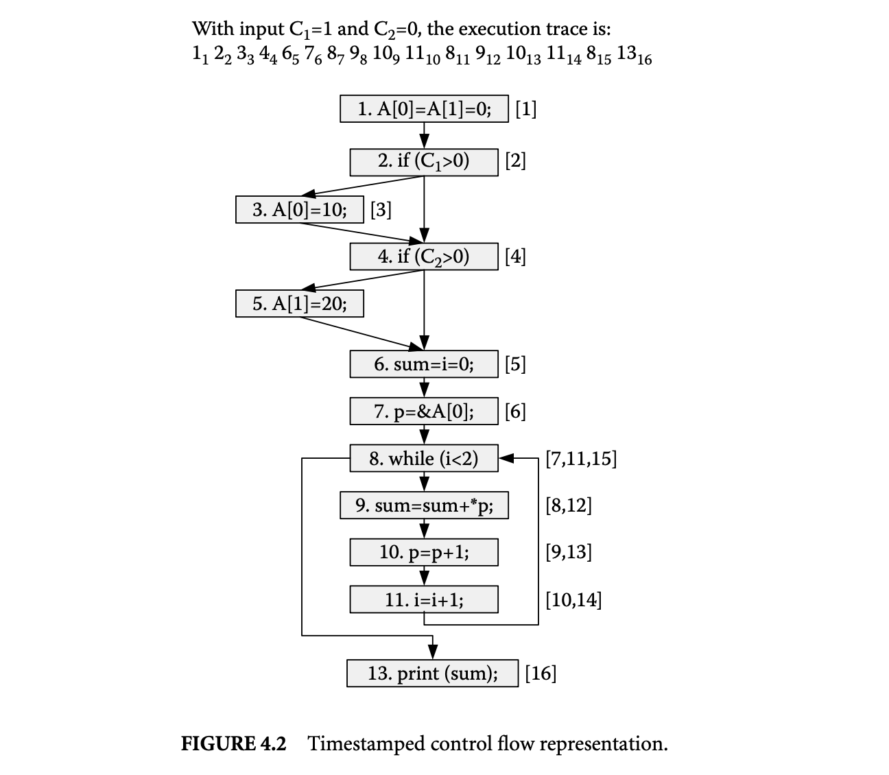
Let's see how the above timestamped representation captures the complete control flow trace. The path taken by the program can be generated from a labeled control flow graph using the combination of static control flow edges and the sequences of timestamps associated with nodes. If a node $n$ is labeled with timestamp value $t$ , the node that is executed next must be the static control flow successor of $n$ that is labeled with timestamp value $t + 1$ . Using this observation, the complete path or part of the program path starting at any execution point can be easily generated.

4.2.1.2 Whole Value Trace

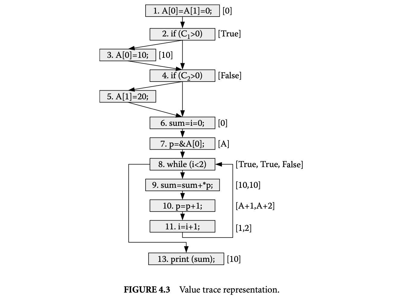
The whole value trace captures all values and addresses computed and referenced by executed statements. Instrumentation code must be introduced for each instruction in the program to collect the value trace for a program run. To represent the control flow trace, with each statement, we already associate a sequence of timestamps $(t_{0}, t_{1}, t_{2}, \dots)$ corresponding to the statement execution instances. To represent the value trace, we also associate a sequence of values $(ν_{0}, ν_{1}, ν_{2}, \dots)$ with the statement. These are the values computed by the statement's execution instances. Hence, there is one-to-one correspondence between the sequence of timestamps and the sequence of values.

Two points are worth noting here. First, by capturing values as stated above, we are actually capturing both values and addresses, as some instructions compute data values while others compute addresses. Second, with each statement, we only associate the result values computed by that statement. We do not explicitly associate the values used as operands by the statement. This is because we can access the operand values by traversing the data dependence edges and then retrieving the values from the value traces of statements that produce these values.

Now let us illustrate the above representation by giving the value traces for the program run considered in Figure 4.2. The sequence of values produced by each statement for this program run is shown in Figure 4.3. For example, statement 11 is executed twice and produces values 1 and 2 during these executions.

4.2.1.3 Whole Dependence Trace

A dependence occurs between a pair of statements; one is the source of the dependence and the other is the destination. Dependence is represented by an edge from the source to the destination in the static control flow graph. There are two types of dependences:

Static data dependence: A statement $d$ is statically data dependent upon statement $s$ if a value computed by statement $s$ may be used as an operand by statement $d$ in some program execution. Static control dependence: A statement $d$ is statically control dependent upon a predicate $s$ if the outcome of predicate $s$ can directly determine whether $d$ is executed in some program execution.

The whole data and control dependence trace captures the dynamic occurrences of all static data and control dependences during a program run. A static edge from the source of a dependence to its destination is labeled with dynamic information to capture each dynamic occurrence of a static dependence during the program run. The dynamic information essentially identifies the execution instances of the source and destination statements involved in a dynamic dependence. Since execution instances of statements are identified by their timestamps, each dynamic dependence is represented by a pair of timestamps that identify the execution instances of statements involved in the dynamic dependence. If a static dependence $s \to d$ is exercised multiple times during a program run, it will be labeled by a sequence of timestamp pairs $([t_{s}^{0}, t_{d}^{0}], [t_{s}^{1}, t_{d}^{1}], \dots)$ corresponding to multiple occurrences of the dynamic dependence observed during the program run.

Let us briefly discuss how dynamic dependences are identified during a program run. To identify dynamic data dependences, we need to further process the address trace. For each memory address the execution instance of an instruction that was responsible for the latest write to the address is remembered. When an execution instance of an instruction uses the value at an address, a dynamic data dependence is established between the execution instance of the instruction that performed the latest write to the address and the execution instance of the instruction that used the value at the address. Dynamic control dependences are also identified. An execution instance of an instruction is dynamically control dependent upon the execution instance of the predicate that caused the execution of the instruction. By first computing the static

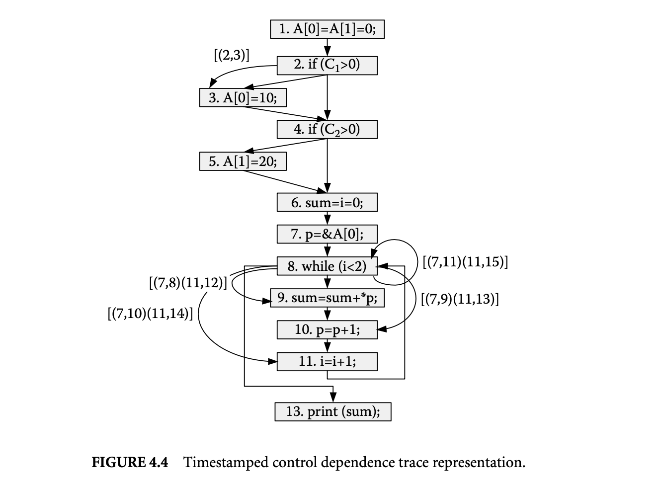
control predecessors of an instruction, and then detecting which one of these was the last to execute prior to a given execution of the instruction from the control flow trace, dynamic control dependences are identified.

Now let us illustrate the above representation by giving the dynamic data and control dependences for the program run considered in Figure 4.2. First let's consider the dynamic control dependences shown in Figure 4.4. The control dependence edges in this program include $2 \to 3$ , $4 \to 5$ , $8 \to 9$ , $8 \to 10$ , and $8 \to 11$ . These edges are labeled with timestamp pairs. The edge $2 \to 3$ is labeled with $([2, 3])$ because this dependence is exercised only once and the timestamps of the execution instances involved are $2$ and $3$ . The edge $4 \to 5$ is not labeled because it is not exercised in the program run. However, edge $8 \to 9$ is labeled with $([7, 8], [11, 12])$ , indicating that this edge is exercised twice. The timestamps in each pair identify the execution instances of statements involved in the dynamic dependences.

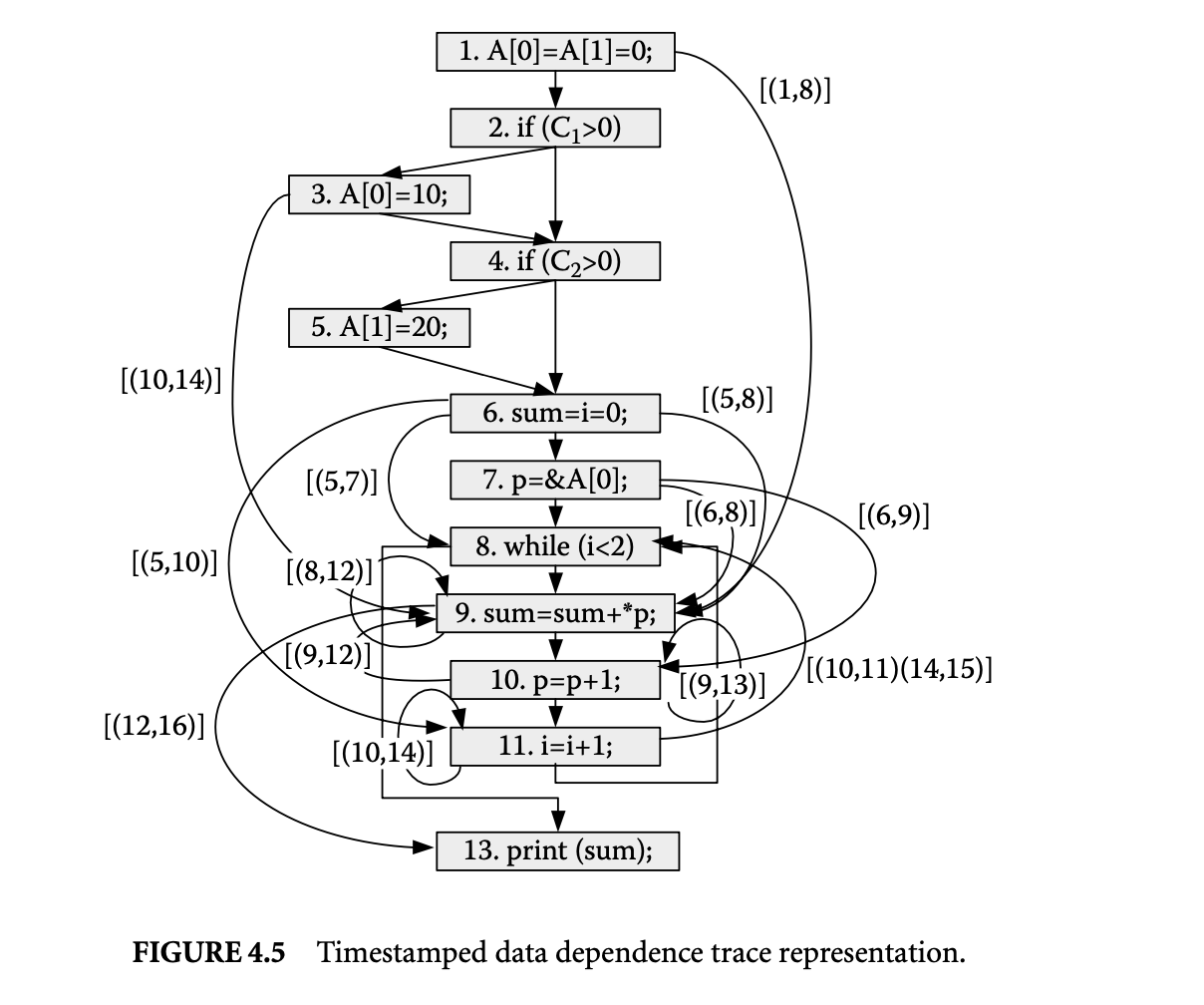
Next let us consider the dynamic data dependence edges shown in Figure 4.5. The darker edges correspond to static data dependence edges that are labeled with sequences of timestamp pairs that capture dynamic instances of data dependences encountered during the program run. For example, edge $11 \to 8$ shows the flow of the value of variable $i$ from its definition in statement 11 to its use in statement 8. This edge is labeled $([10, 11], [14, 15])$ because it is exercised twice in the program run. The timestamps in each pair identify the execution instances of statements involved in the dynamic dependences.

4.2.2 Compressing Whole Execution Traces

Because of the large amount of information contained in WETs, the storage needed to hold the WETs is very large. In this section we briefly outline a two-tier compression strategy for greatly reducing the space requirements.

The first tier of our compression strategy focuses on developing separate compression techniques for each of the three key types of information labeling the WET graph: (a) timestamps labeling the nodes, (b) values labeling the nodes, and (c) timestamp pairs labeling the dependence edges. Let us briefly consider these compression techniques:

Timestamps labeling the nodes: The total number of timestamps generated is equal to the number of basic block executions, and each of the timestamps labels exactly one basic block. We can reduce the

space taken up by the timestamp node labels as follows. Instead of having nodes that correspond to basic blocks, we create a WET in which nodes can correspond to Ball Larus paths [2] that are composed of multiple basic blocks. Since a unique timestamp value is generated to identify the execution of a node, now fewer timestamps will be generated. In other words, when a Ball Larus path is executed, all nodes in the path share the same timestamp. By reducing the number of timestamps, we save space without having any negative impact on the traversal of WET to extract the control flow trace.

Values labeling the nodes: It is well known that subcomputations within a program are often performed multiple times on the same operand values. This observation is the basis for widely studied techniques for reuse-based redundancy removal [18]. This observation can be exploited in devising a compression scheme for sequence of values associated with statements belonging to a node in the WET. The list of values associated with a statement is transformed such that only a list of unique values produced by it is maintained along with a pattern from which the exact list of values can be generated from the list of unique values. The pattern is often shared across many statements. The above technique yields compression because by storing the pattern only once, we are able to eliminate all repetitions of values in value sequences associated with all statements.

Timestamp pairs labeling the dependence edges:: Each dependence edge is labeled with a sequence of timestamp pairs. Next we describe how the space taken by these sequences can be reduced. Our discussion focuses on data dependences; however, similar solutions exist for handling control dependence edges [27]. To describe how timestamp pairs can be reduced, we divide the data dependences into two categories: edges that are local to a Ball Larus path and edges that are nonlocal as they cross Ball Larus path boundaries.

Let us consider a node $n$ that contains a pair of statements $s_{1}$ and $s_{2}$ such that a local data dependence edge exists due to flow of values from $s_{1}$ to $s_{2}$ . For every timestamp pair $(t_{s_{1}}, t_{s_{2}})$ labeling the edge, it is definitely the case that $t_{s_{1}} = t_{s_{2}}$ . In addition, if $s_{2}$ always receives the involved operand value from $s_{1}$ , then we do not need to label this edge with timestamp pairs. This is because the timestamp pairs that label the edge can be inferred from the labels of node $n$ . If node $n$ is labeled with timestamp $t_{n}$ , under the above conditions,

the data dependence edge must be labeled with the timestamp pair $< t_{n}, t_{n} >$ . It should be noted that by creating nodes corresponding to Ball Larus paths, opportunities for elimination of timestamp pair labels increase greatly. This is because many nonlocal edges get converted to local edges.

Let us consider nonlocal edges next. Often multiple data dependence edges are introduced between a pair of nodes. It is further often the case that these edges have identical labels. In this case we can save space by creating a representation for a group of edges and save a single copy of the labels.

For the second-tier compression we view the information labeling the WET as consisting of streams of values arising from the following sources: (a) a sequence of $< t, v >$ pairs labeling a node gives rise to two streams, one corresponding to the timestamps ( $t s$ ) and the other corresponding to the values ( $v s$ ), and (b) a sequence of $< t_{i_{1}}, t_{i_{2}} >$ pairs labeling a dependence edge also gives rise to two streams, one corresponding to the first timestamps ( $t_{i_{1}}$ s) and the other corresponding to the second timestamps ( $t_{i_{2}}$ s). Each of the above streams is compressed using a value-prediction-based algorithm [28].

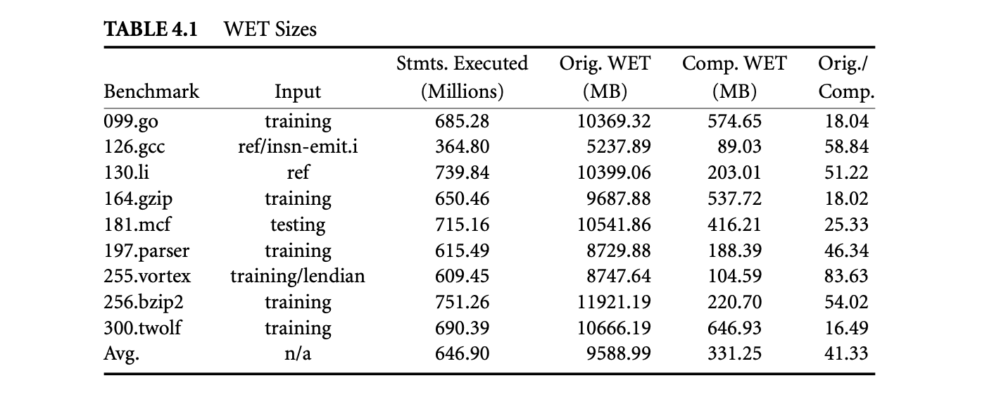
Table 1 lists the benchmarks considered and the lengths of the program runs, which vary from 365 and 751 million intermediate-level statements. WETs could not be collected for complete runs for most benchmarks even though we tried using Trimaran-provided inputs with shorter runs. The effect of our two-tier compression strategy is summarized in Table 1. While the average size of the original uncompressed WETs (Orig. WET) is 9589 megabytes, after compression their size (Comp. WET) is reduced to 331 megabytes, which represents a compression ratio (Orig./Comp.) of 41. Therefore, on average, our approach enables saving of the whole execution trace corresponding to a program run of 647 million intermediate statements using 331 megabytes of storage.

4.3 Using WET in Debugging

In this section we consider two debugging scenarios and demonstrate how WET-based analysis can be employed to assist in fault location in both scenarios. In the first scenario we have a program that fails to produce the correct output for a given input, and it is our goal to assist the programmer in locating the faulty code. In the second scenario we are given two versions of a program that should behave the same but do not do so on a given input, and our goal is to help the programmer locate the point at which the behavior of the two versions diverges. The programmer can then use this information to correct one of the versions.

4.3.1 Dynamic Program Slicing

Let us consider the following scenario for fault location. Given a failed run of a program, our goal is to identify a fault candidate set, that is, a small subset of program statements that includes the faulty code whose execution caused the program to fail. Thus, we assume that the fact that the program has failed is known because either the program crashed or it produced an output that the user has determined to be incorrect. Moreover, this failure is due to execution of faulty code and not due to other reasons (e.g., faulty environment variable setting).

The statements executed during the failing run can constitute a first conservative approximation of the fault candidate set. However, since the user has to examine the fault candidate set manually to locate faulty code, smaller fault candidate sets are desirable. Next we describe a number of dynamic-slicing-based techniques that can be used to produce a smaller fault candidate set than the one that includes all executed statements.

4.3.1.1 Backward Dynamic Slicing

Consider a failing run that produces an incorrect output value or crashes because of dereferencing of an illegal memory address. The incorrect output value or the illegal address value is now known to be related to faulty code executed during this failed run. It should be noted that identification of an incorrect output value will require help from the user unless the correct output for the test input being considered is already available to us. The fault candidate set is constructed by computing the backward dynamic slice starting at the incorrect output value or illegal address value. The backward dynamic slice of a value at a point in the execution includes all those executed statements that effect the computation of that value [1, 14]. In other words, statements that directly or indirectly influence the computation of faulty value through chains of dynamic data and/or control dependences are included in the backward dynamic slices. Thus, the backward reachable subgraph forms the backward dynamic slice, and all statements that appear at least once in the reachable subgraph are contained in the backward dynamic slice. During debugging, both the statements in the dynamic slice and the dependence edges that connect them provide useful clues to the failure cause.

We illustrate the benefit of backward dynamic slicing with an example of a bug that causes a heap overflow error. In this program, a heap buffer is not allocated to be wide enough, which causes an overflow. The code corresponding to the error is shown in Figure 4.6. The heap array $A$ allocated at line 10 overflows at line 11, causing the program to crash. Therefore, the dynamic slice is computed starting at the address of $A [i]$ that causes the segmentation fault. Since the computation of the address involves $A []$ and $i$ , both statements at lines 10 and 10 are included in the dynamic slice. By examining statements at lines 10 and 10, the cause of the failure becomes evident to the programmer. It is easy to see that although a_count entries have been allocated at line 10, b_count entries are accessed according to the loop bounds of the for statement at line 10. This is the cause of the heap overflow at line 11. The main benefit of using dynamic slicing is that it focuses the attention of the programmer on the two relevant lines of code (10 and 10), enabling the fault to be located.

We studied the execution times of computing backward dynamic slices using WETs. The results of this study are presented in Figure 4.7. In this graph each point corresponds to the average dynamic slicing time for 25 slices. For each benchmark 25 new slices are computed after an execution interval of 15 million statements. These slices correspond to 25 distinct memory references. Following each execution interval slices are computed for memory addresses that had been defined since the last execution interval. This was done to avoid repeated computation of the same slices during the experiment. The increase in slicing times is linear with respect to the number of statements executed. More importantly, the slicing times are very promising. For 9 out of 10 benchmarks the average slicing time for 25 slices computed at the end of the run is below 18 seconds. The only exception is 300.twolf, for which the average slicing time at the

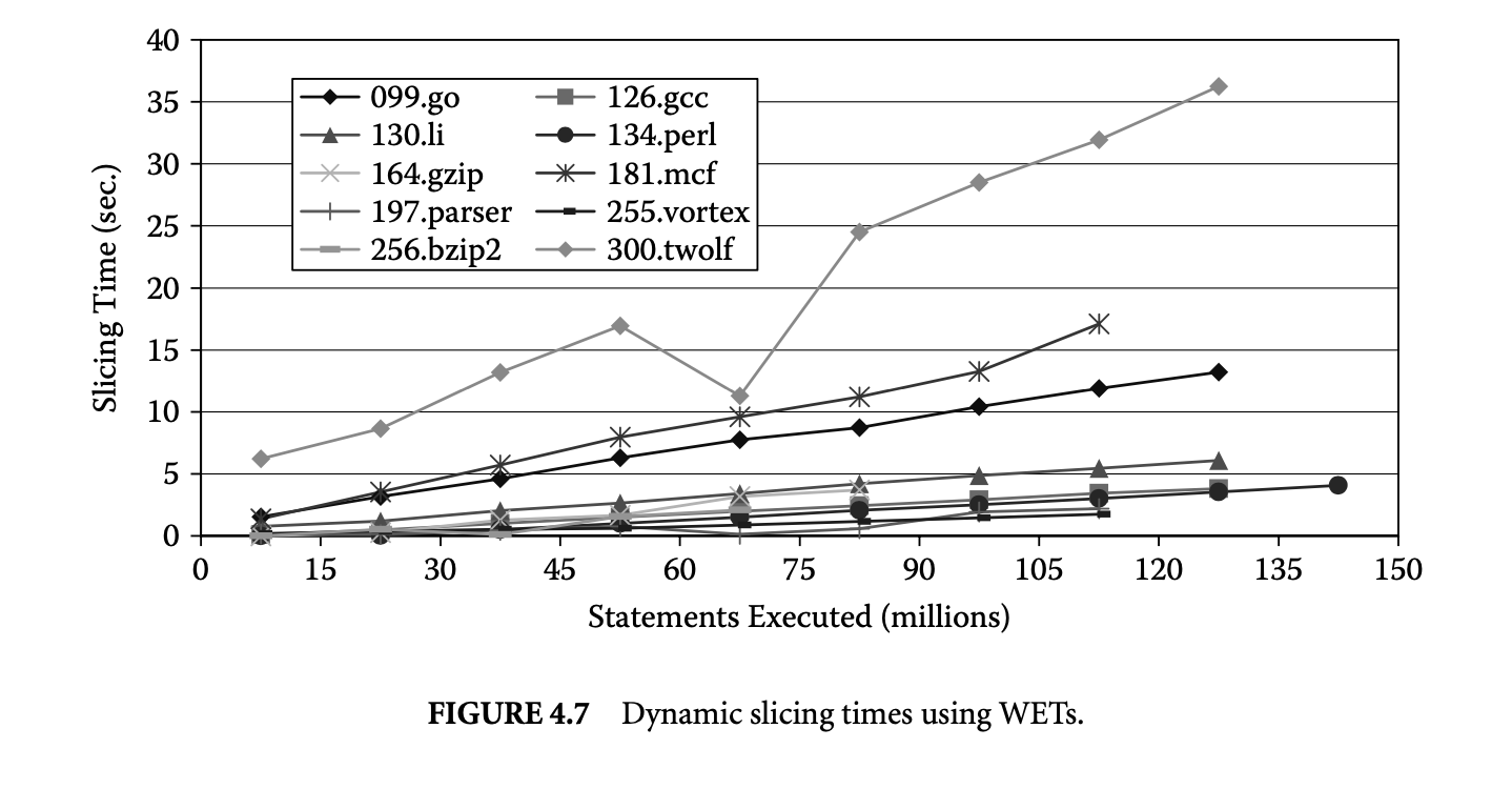end of the program run is roughly 36 seconds. We noted that the compression algorithm did not reduce the graph size for this program as much as many of the other benchmarks. Finally, at earlier points during program runs the slicing times are even lower.

4.3.1.2 Forward Dynamic Slicing

Zeller introduced the term delta debugging[22] for the process of determining the causes of program behavior by looking at the differences (the deltas) between the old and new configurations of the programs. Hildebrandt and Zeller [10, 23] then applied the delta debugging approach to simplify and isolate the failure-inducing input difference. The basic idea of delta debugging is as follows. Given two program runs $r_{s}$ and $r_{f}$ corresponding to the inputs $I_{s}$ and $I_{f}$ , respectively, such that the program fails in run $r_{f}$ and completes execution successfully in run $r_{s}$ , the delta debugging algorithm can be used to systematically produce a pair of inputs $I_{s}^{'}$ and $I_{f}^{'}$ with a minimal difference such that the program fails for $I_{f}^{'}$ and executes successfully for $I_{s}^{'}$ . The difference between these two inputs isolates the failure-inducing difference part of the input. These inputs are such that their values play a critical role in distinguishing a successful run from a failing run.

Since the minimal failure-inducing input difference leads to the execution of faulty code and hence causes the program to fail, we can identify a fault candidate set by computing a forward dynamic slice starting at this input. In other words, all statements that are influenced by the input value directly or indirectly through a chain of data or control dependences are included in the fault candidate set. Thus, now we have a means for producing a new type of dynamic slice that also represents a fault candidate set. We recognized the role of forward dynamic slices in fault location for the first time in [8].

Let us illustrate the use of forward dynamic slicing using the program in Figure 4.8. In this program if the length of the input is longer than 1,024, the writes to Buffer[i] at line 6 overflow the buffer corrupting the pointer stored in CorruptPointer. As a result, when we attempt to execute the free at line 9, the program crashes.

Let us assume that to test the above program we picked the following two inputs: the first input is 'aaaaa', which is a successful input, and the second input is 'a $<$ repeated 2000 times $>^{'}$ , which is a failing input because the length is larger than 1,024. After applying the $s d d mi$ algorithm in [23] on them, we have two new inputs: the new successful input is 'a $<$ repeated 1024 times $>^{'}$ and the new failing input is 'a $<$ repeated 1025 times $>^{'}$ . The failure-inducing input difference between them is the last character 'a' in the new failed input.

Now we compute the forward dynamic slice of 1,025th 'a' in the failing input. The resulting dynamic slice consists of a data dependence chain originating at statement INPUT[i] at line 5, leading to the write to 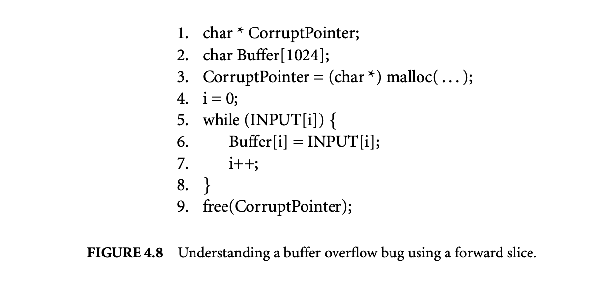Buffer[i] at line 6, and then leading to the statement free(CorruptPointer) at line 9. When the programmer examines this data dependence chain, it becomes quite clear that there is an unexpected data dependence from Buffer[i] at line 6 to free(CorruptPointer) at line 9. Therefore, the programmer can conclude that Buffer[i] has overflowed. This is the best result one can expect from a fault location algorithm. This is because, other than the input statement, the forward dynamic slice captures exactly two statements. These are the two statements between which the spurious data dependence was established, and hence they must be minimally present in the fault candidate set.

4.3.1.3 Bidirectional Dynamic Slicing

Given an erroneous run of the program, the objective of this method is to explicitly force the control flow of the program along an alternate path at a critical branch predicate such that the program produces the correct output. The basic idea of this approach is inspired by the following observation. Given an input on which the execution of a program fails, a common approach to debugging is to run the program on this input again, interrupt the execution at certain points to make changes to the program state, and then see the impact of changes on the continued execution. If we can discover the changes to the program state that cause the program to terminate correctly, we obtain a good idea of the error that otherwise was causing the program to fail. However, automating the search of state changes is prohibitively expensive and difficult to realize because the search space of potential state changes is extremely large (e.g., even possible changes for the value of a single variable are enormous if the type of the variable is integer or float). However, changing the outcomes of predicate instances greatly reduces the state search space since a branch predicate has only two possible outcomes: true or false. Therefore, we note that through forced switching of the outcomes of some predicate instances at runtime, it may be possible to cause the program to produce correct results.

Having identified a critical predicate instance, we compute a fault candidate set as the bidirectional dynamic slice of the critical predicate instance. This bidirectional dynamic slice is essentially the union of the backward dynamic slice and the forward dynamic slice of the critical predicate instance. Intuitively, the reason the slice must include both the backward and forward dynamic slice is as follows. Consider the situation in which the effect of executing faulty code is to cause the predicate to evaluate incorrectly. In this case the backward dynamic slice of the critical predicate instance will capture the faulty code. However, it is possible that by changing the outcome of the critical predicate instance we avoid the execution of faulty code, and hence the program terminates normally. In this case the forward dynamic slice of the critical predicate instance will capture the faulty code. Therefore, the faulty code will be in either the backward dynamic slice or the forward dynamic slice. We recognized the role of bidirectional dynamic slices in fault location for the first time in [26], where more details on identification of the critical predicate instance can also be found.

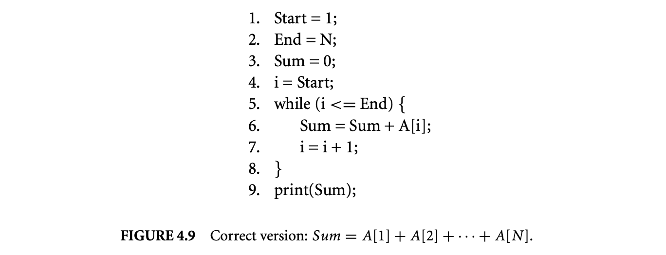
Next we present an example to illustrate the need for bidirectional dynamic slices. We consider a simple program shown in Figure 4.9 that sums up the elements of an array $(A [1] + A [2] + \dots + A [N])$ . While this is the correct version of the program, next we will create three faulty versions of this program. In each of these versions the critical predicate instance can be found. However, the difference in these versions is where in the bidirectional dynamic slice the faulty code is present, that is, the critical predicate, the backward dynamic slice of the critical predicate, and the forward dynamic slice of the critical predicate:

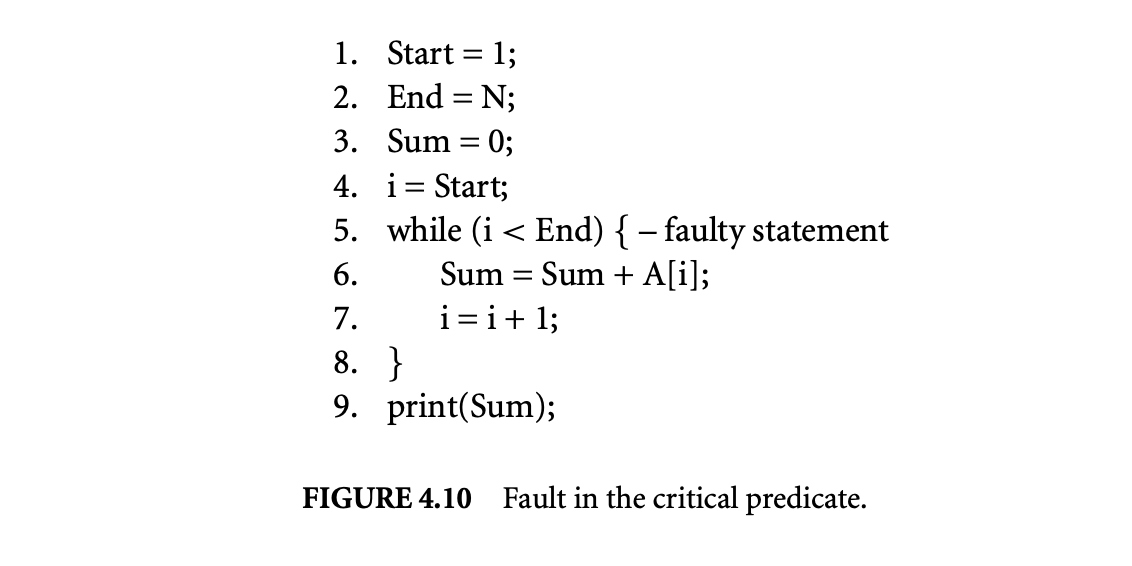
Fault in the critical predicate:: Figure 4.10 shows a faulty version of the program from Figure 4.9. In this faulty version, the error in the predicate of the while loop results in the loop executing for one fewer iterations. As a result, the value of $A [N]$ is not added to Sum, producing an incorrect output. The critical predicate instance identified for this program run is the last execution instance of the while loop predicate. This is because if the outcome of the last execution instance of the while loop predicate is switched from false to true, the loop iterates for another iteration and the output produced by the program becomes correct. Given this information, the programmer can ascertain that the error is in the while loop predicate, and it can be corrected by modifying the relational operator from $<$ to $<=$ . 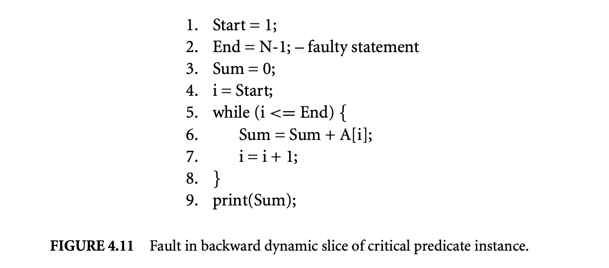Fault in the backward dynamic slice of the critical predicate instance:: In the previous faulty version, the critical predicate identified was itself faulty. Next we show that in a slightly altered version of the faulty version, the fault is not present in the critical predicate but rather in the backward dynamic slice of the critical predicate. Figure 4.11 shows this faulty version. The fault is in the initialization of End at line 3, and this causes the while loop to execute for one fewer iterations. Again, the value of $A [N]$ is not added to Sum, producing an incorrect output. The critical predicate instance identified for this program run is the last execution instance of the while loop predicate. This is because if the outcome of the last execution instance of the while loop predicate is switched from false to true, the loop iterates for another iteration and the output produced by the program becomes correct. However, in this situation the programmer must examine the backward dynamic slice of the critical predicate to locate the faulty initialization of End at line 3. 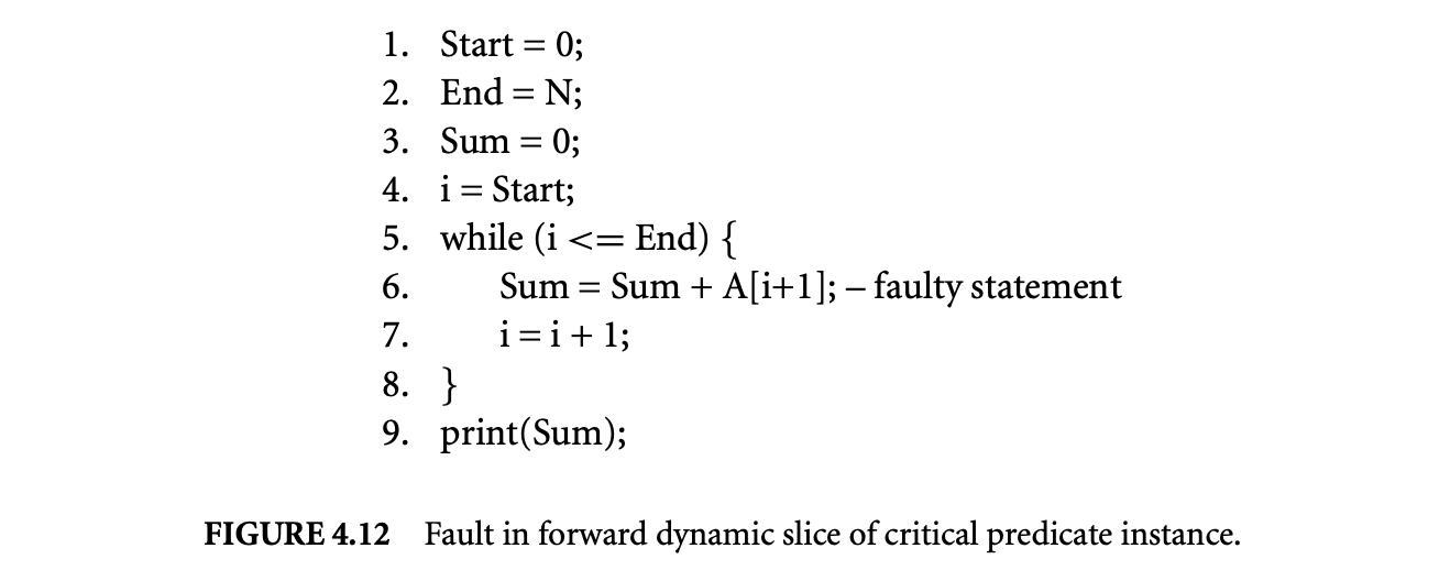Fault in the forward dynamic slice of the critical predicate instance:: Finally, we show a faulty version in which the faulty code is present in the forward dynamic slice of the critical predicate instance. Figure 4.12 shows this faulty version. The fault is at line 6, where reference to $A [i + 1]$ should bereplaced by reference to $A [i]$ .

When this faulty version is executed, let us consider the situation in which when the last loop iteration is executed, the reference to $A [N + 1]$ at line 6 causes the program to produce a segmentation fault. The most recent execution instance of the while loop predicate is evaluated to true. However, if we switch this evaluation to false, the loop executes for one fewer iterations, causing the program crash to disappear. Note that the output produced is still incorrect because the value of $A [1]$ is not added to Sum. However, since the program no longer crashes, the programmer can analyze the program execution to understand why the program crash is avoided. By examining the forward dynamic slice of the critical predicate instance, the programmer can identify the statements, which when not executed avoid the program crash. This leads to the identification of reference to $A [i + 1]$ as the fault.

In the above discussion we have demonstrated that once the critical predicate instance is found, the fault may be present in the critical predicate, its backward dynamic slice, or its forward dynamic slice. Of course, the programmer does not know beforehand where the fault is. Therefore, the programmer must examine the critical predicate, the statements in the backward dynamic slice, and the statements in the forward dynamic slice one by one until the faulty statement is found.

4.3.1.4 Pruning Dynamic Slices

In the preceding discussion we have shown three types of dynamic slices that represent reduce fault candidate sets. In this section we describe two additional techniques for further pruning the sizes of the fault candidate sets:

Coarse-grained pruning:: When multiple estimates of fault candidate sets are found using backward, forward, and bidirectional dynamic slices, we can obtain a potentially smaller fault candidate set by intersecting the three slices. We refer to this simple approach as the coarse-grained pruning approach. In [24] we demonstrate the benefits of this approach by applying it to a collection of real bugs reported by users. The results are very encouraging, as in many cases the fault candidate set contains only a handful of statements. Fine-grained pruning: In general, it is not always possible to compute fault candidate sets using backward, forward, and bidirectional dynamic slices. For example, if we fail to identify a minimal failure-inducing input difference and a critical predicate instance, then we cannot compute the forward and bidirectional dynamic slices. As a result, coarse-grained pruning cannot be applied. To perform pruning in such situations we developed a fine-grained pruning technique that reduces the fault candidate set size by eliminating statements in the backward dynamic slice that are expected not to be faulty.

The fine-grained pruning approach is based upon value profiles of executed statements. The main idea behind this approach is to exploit correct outputs produced during a program run before an incorrect output is produced or the program terminates abnormally. The executed statements and their value profiles are examined to find likely correct statements in the backward slice. These statements are such that if they are altered, they will definitely cause at least one correct output produced during the program run to change. All statements that fall in this category are marked as likely correct and thus pruned from the backward dynamic slice. The detailed algorithm can be found in [25] along with experimental data that show that this pruning approach is highly effective in reducing the size of the fault candidate set. It should be noted that this fine-grained pruning technique makes use of both dependence and value traces contained in the WET.

4.3.2 Dynamic Matching of Program Versions

Now we consider a scenario in which we have two versions of a program such that the second version has been derived through application of transformations to the first version. When the two versions are executed on an input, it is found that while the first version runs correctly, the second version does not. In such a situation it is useful to find out the execution point at which the dynamic behavior of the two versions deviates, since this gives us a clue to the cause of differing behaviors.

The above scenario arises in the context of optimizing compilers. Although compile-time optimizations are important for improving the performance of programs, applications are typically developed with the optimizer turned off. Once the program has been sufficiently tested, it is optimized prior to its deployment. However, the optimized program may fail to execute correctly on an input even though the unoptimized program ran successfully on that input. In this situation the fault may have been introduced by the optimizer through the application of an unsafe optimization, or a fault present in the original program may have been exposed by the optimizations. Determining the source and cause of the fault is therefore important.

In [12] a technique called comparison checking was proposed to address the above problem. A comparison checker executes the optimized and unoptimized programs and continuously compares the results produced by corresponding instruction executions from the two versions. At the earliest point during execution at which the results differ, they are reported to the programmer, who can use this information to isolate the cause of the faulty behavior. It should be noted that not every instruction in one version has a corresponding instruction in the other version because optimizations such as reassociation may lead to instructions that compute different intermediate results. While the above approach can be used to test optimized code thoroughly and assist in locating a fault if one exists, it has one major drawback. For the comparison checker to know which instruction executions in the two versions correspond to each other, the compiler writer must write extra code that determines mappings between execution instances of instructions in the two program versions. Not only do we need to develop a mapping for each kind of optimization to capture the effect of that optimization, but we must also be able to compose the mappings for different optimizations to produce the mapping between the unoptimized and fully optimized code. The above task is not only difficult and time consuming, but it must be performed each time a new optimization is added to the compiler.

We have developed a WET-based approach for automatically generating the mappings. The basic idea behind our approach is to run the two versions of the programs and regularly compare their execution histories. The goal of this comparison is to find matches between the execution history of each instruction in the optimized code with execution histories of one or more instructions in the unoptimized code.

If execution histories match closely, it is extremely likely that they are indeed the corresponding instructions in the two program versions. At each point when executions of the programs are interrupted, their histories are compared with each other. Following the determination of matches, we determine if faulty behavior has already manifested itself, and accordingly potential causes of faulty behavior are reported to the user for inspection. For example, instructions in the optimized program that have been executed numerous times but do not match anything in the unoptimized code can be reported to the user for examination. In addition, instructions that matched each other in an earlier part of execution but later did not match can be reported to the user. This is because the later phase of execution may represent instruction executions after faulty behavior manifests itself. The user can then inspect these instructions to locate the fault(s).

The key problem we must solve to implement the above approach is to develop a matching process that is highly accurate. We have designed a WET-based matching algorithm that consists of the following two steps: signature matching and structure matching. A signature of an instruction is defined in terms of the frequency distributions of the result values produced by the instruction and the addresses referenced by the instruction. If signatures of two instructions are consistent with each other, we consider them to tentatively match. In this second step we match the structures of the data dependence graphs produced by the two versions. Two instructions from the two versions are considered to match if there was a tentative signature match between them and the instructions that provided their operands also matched with each other.

In the Trimaran system [19] we generated two versions of very long instructional word (VIW) machine code supported under the Trimaran system by generating an unoptimized and an optimized version of programs. We ran the two versions on the same input and collected their detailed whole execution traces. The execution histories of corresponding functions were then matched. We found that our matching algorithm was highly accurate and produced the matches in seconds [29]. To study the effectiveness of matching for comparison checking as discussed above, we created another version of the optimized code by manually injecting an error in the optimized code. We plotted the number of distinct instructions for which no match was found as a fraction of distinct executed instructions over time in two situations: when the optimized program had no error and when it contained an error. The resulting plot is shown in Figure 4.13. The points in the graph are also annotated with the actual number of instructions in the optimized code for which no match was found. The interval during which an error point is encountered during execution is marked in the figure.

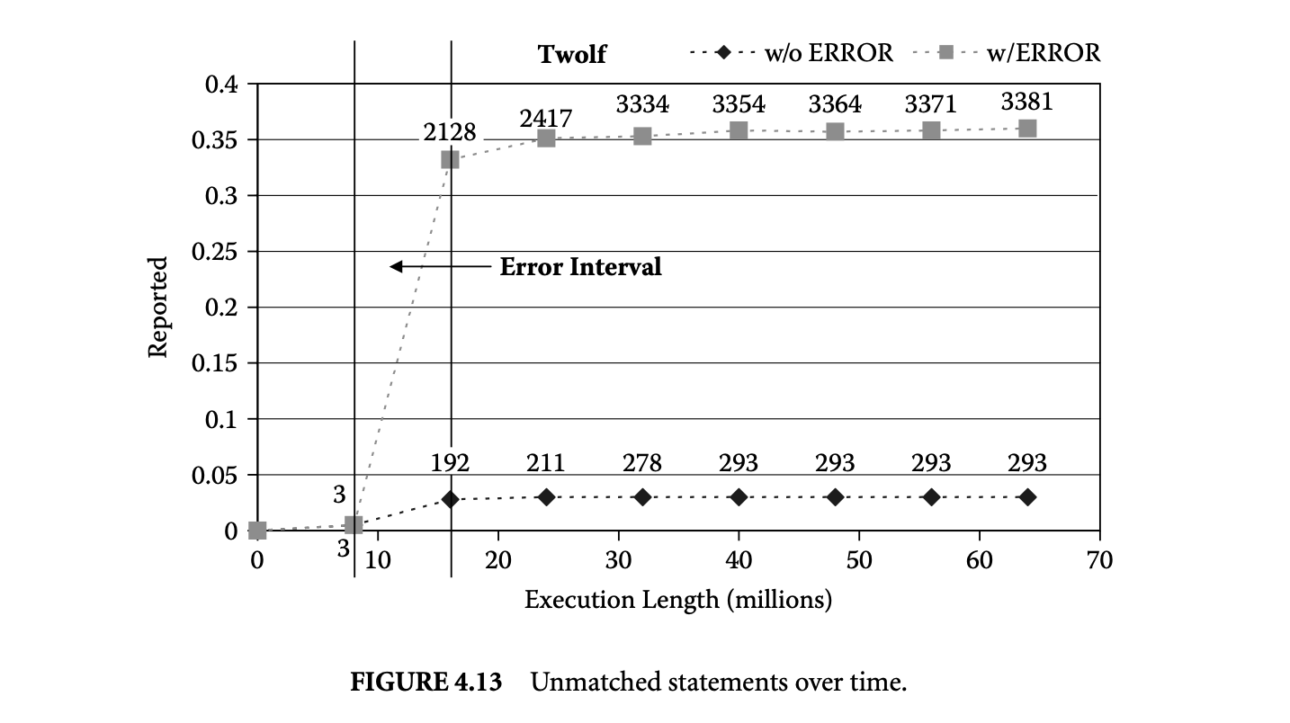
Compared to the optimized program without error, the number of unmatched instructions increases sharply after the error interval point is encountered. The increase is quite sharp -- from 3 to 35%. When we look at the actual number of instructions reported immediately before and after the execution interval during which the error is first encountered, the number reported increases by an order of magnitude.

By examining the instructions in the order they are executed, erroneous instructions can be quickly isolated. Other unmatched instructions are merely dependent upon the instructions that are the root causes of the errors. Out of the over 2,000 unmatched instructions at the end of the second interval, we only need to examine the first 15 unmatched instructions in temporal order to find an erroneous instruction.

4.4 Concluding Remarks

The emphasis of earlier research on profiling techniques was separately studying single types of profiles (control flow, address, value, or dependence) and capturing only a subset of profile information of a given kind (e.g., hot control flow paths, hot data streams). However, recent advances in profiling enable us to simultaneously capture and compactly represent complete profiles of all types. In this chapter we described the WET representation that simultaneously captures complete profile information of several types of profile data. We demonstrated how such rich profiling data can serve as the basis of powerful dynamic analysis techniques. In particular, we described how dynamic slicing and dynamic matching can be performed efficiently and used to greatly assist a programmer in locating faulty code under two debugging scenarios.

References

H. Agrawal and J. Horgan. 1990. Dynamic program slicing. In ACM SIGPLAN Conference on Programming Language Design and Implementation, 246-56. New York, NY: ACM Press.
T. Ball and J. Larus. 1996. Efficient path profiling. In IEEE/ACM International Symposium on Microarchitecture, 46-57. Washington, DC, IEEE Computer Society.
R. Bodik, R. Gupta, and M. L. Soffa. 1998. Complete removal of redundant expressions. In ACM SIGPLAN Conference on Programming Language Design and Implementation, 1-14, Montreal, Canada. New York, NY: ACM Press.
M. Burtscher and M. Jeeradit. 2003. Compressing extended program traces using value predictors. In International Conference on Parallel Architectures and Compilation Techniques, 159-69. Washington, DC, IEEE Computer Society.
B. Calder, P. Feller, and A. Eustace. 1997. Value profiling. In IEEE/ACM International Symposium on Microarchitecture, 259-69. Washington, DC, IEEE Computer Society.
T. M. Chilimbi. 2001. Efficient representations and abstractions for quantifying and exploiting data reference locality. In ACM SIGPLAN Conference on Programming Language Design and Implementation, 191-202, Snowbird, UT. New York, NY: ACM Press.
T. M. Chilimbi and M. Hirzel. 2002. Dynamic hot data stream prefetching for general-purpose programs. In ACM SIGPLAN Conference on Programming Language Design and Implementation, 199-209. New York, NY: ACM Press.
N. Gupta, H. He, X. Zhang, and R. Gupta. 2005. Locating faulty code using failure-inducing chops. In IEEE/ACM International Conference on Automated Software Engineering, 263-72, Long Beach, CA. New York, NY: ACM Press.
R. Gupta, D. Berson, and J. Z. Fang. 1998. Path profile guided partial redundancy elimination using speculation. In IEEE International Conference on Computer Languages, 230-39, Chicago, IL. Washington, DC, IEEE Computer Society.
R. Hildebrandt and A. Zeller. 2000. Simplifying failure-inducing input. In International Symposium on Software Testing and Analysis, 135-45. New York, NY: ACM Press.
Q. Jacobson, E. Rotenberg, and J. E. Smith. 1997. Path-based next trace prediction. In IEEE/ACM International Symposium on Microarchitecture, 14-23. Washington, DC, IEEE Computer Society.
C. Jaramillo, R. Gupta, and M. L. Soffa. 1999. Comparison checking: An approach to avoid debugging of optimized code. In ACM SIGSOFT 7th Symposium on Foundations of Software Engineering and 8th European Software Engineering Conference. LNCS 1687, 268-84. Heidelberg, Germany: Springer-Verlag. New York, NY: ACM Press.
D. Joseph and D. Grunwald. 1997. Prefetching using Markov predictors. In International Symposium on Computer Architecture, 252-63. New York, NY: ACM Press.
B. Korel and J. Laski. 1988. Dynamic program slicing. Information Processing Letters, 29(3): 155-63. Amsterdam, The Netherlands: Elsevier North-Holland, Inc.
J. R. Larus. 1999. Whole program paths. In ACM SIGPLAN Conference on Programming Language Design and Implementation, 259-69, Atlanta, GA. New York, NY: ACM Press.
M. H. Lipasti and J. P. Shen. 1996. Exceeding the dataflow limit via value prediction. In IEEE/ACM International Symposium on Microarchitecture, 226-37. Washington, DC, IEEE Computer Society.
S. Rubin, R. Bodik, and T. Chilimbi. 2002. An efficient profile-analysis framework for data layout optimizations. In ACM SIGPLAN-SIGACT Symposium on Principles of Programming Languages, 140-53, Portland, OR. New York, NY: ACM Press.
Y. Sazeides. 2003. Instruction-isomorphism in program execution. Journal of Instruction Level Parallelism, 5:1-22.
L. N. Chakrapani, J. Gyllenhaal, W. Hwu, S. A. Mahlke, K. V. Palem, and R. M. Rabbah, Trimaran: An infrastructure for research in instruction-level parallelism, languages, and compliers for high performance computing 2004, LNCS 8602, 32-41, Berlin: Springer/Heidlberg.
J. Yang and R. Gupta. 2002. Frequent value locality and its applications. ACM Transactions on Embedded Computing Systems, 1(1):79-105. New York, NY: ACM Press.
C. Young and M. D. Smith. 1998. Better global scheduling using path profiles. In IEEE/ACM International Symposium on Microarchitecture, 115-23. Washington, DC, IEEE Computer Society.
A. Zeller. 1999. Yesterday, my program worked. Today, it does not. Why? In ACM SIGSOFT Seventh Symposium on Foundations of Software Engineering and Seventh European Software Engineering Conference, 253-67. New York, NY: ACM Press.
A. Zeller and R. Hildebrandt. 2002. Simplifying and isolating failure-inducing input. IEEE Transactions on Software Engineering, 28(2):183-200. Washington, DC, IEEE Computer Society.
Practice & Experience_, vol 37, Issue 9, pp. 935-961, July 2007. New York, NY: John Wiley & Sons, Inc.
X. Zhang, N. Gupta, and R. Gupta. 2006. Pruning dynamic slices with confidence. In ACM SIGPLAN Conference on Programming Language Design and Implementation, 169-80, Ottawa, Canada. New York, NY: ACM Press.
X. Zhang, N. Gupta, and R. Gupta. 2006. Locating faults through automated predicate switching. In International Conference on Software Engineering, 272-81, Shanghai, China. New York, NY: ACM Press.
X. Zhang and R. Gupta. 2004. Cost effective dynamic program slicing. In ACM SIGPLAN Conference on Programming Language Design and Implementation, 94-106, Washington, DC. New York, NY: ACM Press.
X. Zhang and R. Gupta. 2005. Whole execution traces and their applications. ACM Transactions on Architecture and Code Optimization, 2(3):301-34. New York, NY: ACM Press.
X. Zhang and R. Gupta. 2005. Matching execution histories of program versions. In Joint 10th European Software Engineering Conference and ACM SIGSOFT 13th Symposium on Foundations of Software Engineering, 197-206, Lisbon, Portugal. New York, NY: ACM Press.
Y. Zhang and R. Gupta. 2001. Timestamped whole program path representation and its applications. In ACM SIGPLAN Conference on Programming Language Design and Implementation, 180-90, Snowbird, UT. New York, NY: ACM Press.
Y. Zhang and R. Gupta. 2002. Data compression transformations for dynamically allocated data structures. In International Conference on Compiler Construction, Grenoble, France. London, UK: Springer-Verlag.
C. B. Zilles and G. Sohi. 2000. Understanding the backward slices of performance degrading instructions. In ACM/IEEE 27th International Symposium on Computer Architecture, 172-81. New York, NY: ACM Press.

compiler-handbook